Note
This tutorial was generated from an IPython notebook that can be
downloaded here.
Try a live version: ![]() , or view in nbviewer.
, or view in nbviewer.
Regression model fitting
Standard imports
First, setup some standard modules and matplotlib.
[1]:
%matplotlib inline
%config InlineBackend.figure_format = 'png'

import numpy as np
import xarray as xr

import matplotlib.pyplot as plt
Load the main sciapy module and its wrappers for easy access to the used proxy timeseries.
[2]:
import regressproxy
import sciapy
from sciapy.regress.load_data import load_dailymeanAE, load_dailymeanLya
[3]:
plt.rcParams["figure.dpi"] = 120
plt.rcParams["mathtext.default"] = "regular"
Model interface
The model is set up part by part, beginning with the more involved proxy models.
We set some scaling parameters first. The data_scale scales the NO data (~ \(10^7...10^9\) cm\(^{-3}\)) to 1…1000 to avoid possible overflows in the calculations.
[4]:
data_scale = 1e-6
max_days = 100
max_amp = 1e10 * data_scale
Lyman-\(\alpha\) proxy
We start with the Lyman-\(\alpha\) proxy, it is not centered (mean-subtracted) and we set the rest of the parameters except ltscan to zero. This time we also set the bounds for the prior probabilities.
[5]:
# load proxy data
plat, plap = load_dailymeanLya()
# setup the model
lya_model = regressproxy.ProxyModel(plat,
                                    plap["Lya"],
                                    center=False,
                                    amp=0,
                                    lag=0,
                                    tau0=0,
                                    taucos1=0, tausin1=0,
                                    taucos2=0, tausin2=0,
                                    ltscan=60,
                                    bounds={"amp": [-max_amp, max_amp],
                                            "lag": [0, max_days],
                                            "tau0": [0, max_days],
                                            "taucos1": [-max_days, max_days],
                                            "tausin1": [-max_days, max_days],
                                            # semi-annual cycles for the life time
                                            "taucos2": [-max_days, max_days],
                                            "tausin2": [-max_days, max_days],
                                            "ltscan": [0, 200],
                                           },
                                   )
AE proxy with lifetime
The AE proxy is also not centered and we start with the same parameters as above.
[6]:
# load proxy data
paet, paep = load_dailymeanAE()
# setup the model
ae_model = regressproxy.ProxyModel(paet,
                                   paep["AE"],
                                   center=False,
                                   amp=0,
                                   lag=0,
                                   tau0=0,
                                   taucos1=0, tausin1=0,
                                   taucos2=0, tausin2=0,
                                   ltscan=60,
                                   bounds={"amp": [0, max_amp],
                                           "lag": [0, max_days],
                                           "tau0": [0, max_days],
                                           "taucos1": [-max_days, max_days],
                                           "tausin1": [-max_days, max_days],
                                           # semi-annual cycles for the life time
                                           "taucos2": [-max_days, max_days],
                                           "tausin2": [-max_days, max_days],
                                           "ltscan": [0, 200],
                                          },
                                  )
Offset
We use the ConstantModel (inherited from celerite) for the constant offset.
[7]:
offset_model = regressproxy.ConstantModel(value=0.,
                                          bounds={"value": [-max_amp, max_amp]})
Optional harmonic terms
The harmonic terms are not used here but we include them to show how to set them up.
[8]:
harm1 = regressproxy.HarmonicModelCosineSine(freq=1, cos=0, sin=0,
                                             bounds={"cos": [-max_amp, max_amp],
                                                     "sin": [-max_amp, max_amp]})
harm2 = regressproxy.HarmonicModelCosineSine(freq=2, cos=0, sin=0,
                                             bounds={"cos": [-max_amp, max_amp],
                                                     "sin": [-max_amp, max_amp]})

# frequencies should not be fitted
harm1.freeze_parameter("freq")
harm2.freeze_parameter("freq")
Combined model
Together the above models make up the “mean” model we use later together with a Gaussian Process covariance matrix for fitting.
[9]:
model = regressproxy.ProxyModelSet([("offset", offset_model),
                                    ("Lya", lya_model), ("GM", ae_model),
                                    ("f1", harm1), ("f2", harm2)])
The full model has the following parameters:
[10]:
model.get_parameter_dict()
[10]:
OrderedDict([('offset:value', 0.0),
             ('Lya:amp', 0.0),
             ('Lya:lag', 0.0),
             ('Lya:tau0', 0.0),
             ('Lya:taucos1', 0.0),
             ('Lya:tausin1', 0.0),
             ('Lya:taucos2', 0.0),
             ('Lya:tausin2', 0.0),
             ('Lya:ltscan', 60.0),
             ('GM:amp', 0.0),
             ('GM:lag', 0.0),
             ('GM:tau0', 0.0),
             ('GM:taucos1', 0.0),
             ('GM:tausin1', 0.0),
             ('GM:taucos2', 0.0),
             ('GM:tausin2', 0.0),
             ('GM:ltscan', 60.0),
             ('f1:cos', 0.0),
             ('f1:sin', 0.0),
             ('f2:cos', 0.0),
             ('f2:sin', 0.0)])
But we don’t need all of them, so we freeze all parameters and thaw the ones we need. This is easier than the other way around (freezing all unused parameters).
[11]:
model.freeze_all_parameters()
model.thaw_parameter("offset:value")
model.thaw_parameter("Lya:amp")
model.thaw_parameter("GM:amp")
model.thaw_parameter("GM:tau0")
model.thaw_parameter("GM:taucos1")
model.thaw_parameter("GM:tausin1")
Cross check that only the used parameters are really active:
[12]:
model.get_parameter_dict()
[12]:
OrderedDict([('offset:value', 0.0),
             ('Lya:amp', 0.0),
             ('GM:amp', 0.0),
             ('GM:tau0', 0.0),
             ('GM:taucos1', 0.0),
             ('GM:tausin1', 0.0)])
Data
We now load some real data, and we set the latitude and altitude first. The full daily zonal mean data set has the following dimensions:
- altitude: 60, 62, 64, …, 86, 88, 90 [km]
- latitude: -85, -75, -65, …, 65, 75, 85 [°N]
(We have prepared a single timeseries including only the particular altitude and latitude bin to save bandwidth, see below.)
[13]:
altitude = 70  # [km]
latitude = 65  # [°N] geomagn.
We define some helper functions to load the data we need, using the requests module to access online resources in the case the file is not available locally. load_timeseries_store() interfaces xarray.open_dataset with some default chunks set up, selects the altitude and latitude bin and limits the data set to a subset of the variables if set. This function can be used with regular files and with xarray.backends as illustrated in load_timeseries_url().
[14]:
import requests
import netCDF4

def load_timeseries_store(store, alt, lat, variables=None):
    with xr.open_dataset(store, chunks={"latitude": 9, "altitude": 17}) as data_ds:
        data_ts = data_ds.sel(altitude=alt, latitude=lat)
        if variables is not None:
            data_ts = data_ts[variables]
        data_ts.load()
        return data_ts

def load_timeseries_url(url, alt, lat, variables=None):
    with requests.get(url, stream=True) as response:
        nc4_ds = netCDF4.Dataset("data", memory=response.content)
        store = xr.backends.NetCDF4DataStore(nc4_ds)
        return load_timeseries_store(store, alt, lat, variables)
We load the daily zonal mean timeseries from google drive which contains only the above altitude and latitude bin for demonstration purposes. Alternatively, the full zonal mean data set on zenodo could be used directly, but be aware that this transfers the whole file (~600 MB) everytime the cell is executed. However, only a minor fraction of it is used as data_ts.
Another way is to download the file, save it alongisde this notebook, and access it via load_timeseries_store().
The full daily zonal mean timeseries is part of the data set available at
https://zenodo.org/record/1342701 ![]()
[15]:
# the zenodo direct download url (~600 MB!) is:
# "https://zenodo.org/record/1342701/files/scia_nom_dzmNO_2002-2012_v6.2.1_2.2_akm0.002_geomag10_nw.nc"
# the smaller timeseries on google drive:
url = "https://drive.google.com/uc?id=1oA0EDq9KEzKv2QAHXSXCP0EpepM2rfMi&export=download"

# setting the altitude and latitude is not really necessary,
# but is left in here to show how it works.
data_ts = load_timeseries_url(url, altitude, latitude, ["NO_DENS", "NO_DENS_std", "NO_DENS_cnt", "NO_AKDIAG"])
data_ts contains the selected variables of one altitude-latitude bin:
[16]:
data_ts
[16]:
<xarray.Dataset>
Dimensions:      (time: 3401)
Coordinates:
  * time         (time) datetime64[ns] 2002-08-02 2002-08-03 ... 2012-04-08
    altitude     float32 70.0
    latitude     float64 65.0
Data variables:
    NO_DENS      (time) float64 6.105e+07 6.432e+07 ... 6.499e+07 4.545e+07
    NO_DENS_std  (time) float64 3.757e+07 3.526e+07 ... 3.622e+07 2.889e+07
    NO_DENS_cnt  (time) float64 45.0 53.0 59.0 51.0 54.0 ... 52.0 48.0 55.0 28.0
    NO_AKDIAG    (time) float64 0.097 0.06467 0.06016 ... 0.09006 0.09079
Attributes:
    version:            2.2
    L2_data_version:    v6.2_fit_noem_apriori
    creation_time:      Mon Oct 09 2017 10:12:25 +00:00 (UTC)
    author:             Stefan Bender
    binned_on:          Thu Nov 16 2017 09:49:40 UTC+00:00
    latitude_bin_type:  geomagnetic
We exclude some untrustworthy data based on the average averaging kernel diagonal elements. The threshold (0.01) is arbitrary and meant to only show how it works in principle, but it should not be too large to leave at least some of the data. Too small values may include data that are too much influenced by the apriori during the retrieval step. Drop tells where() to leave out the non-useful data instead of masking it with nans.
[17]:
data_ts = data_ts.where(data_ts.NO_AKDIAG > 0.01, drop=True)
The timeseries is now a little shorter (note the changed time dimension):
[18]:
data_ts
[18]:
<xarray.Dataset>
Dimensions:      (time: 3384)
Coordinates:
  * time         (time) datetime64[ns] 2002-08-02 2002-08-03 ... 2012-04-08
    altitude     float32 70.0
    latitude     float64 65.0
Data variables:
    NO_DENS      (time) float64 6.105e+07 6.432e+07 ... 6.499e+07 4.545e+07
    NO_DENS_std  (time) float64 3.757e+07 3.526e+07 ... 3.622e+07 2.889e+07
    NO_DENS_cnt  (time) float64 45.0 53.0 59.0 51.0 54.0 ... 52.0 48.0 55.0 28.0
    NO_AKDIAG    (time) float64 0.097 0.06467 0.06016 ... 0.09006 0.09079
Attributes:
    version:            2.2
    L2_data_version:    v6.2_fit_noem_apriori
    creation_time:      Mon Oct 09 2017 10:12:25 +00:00 (UTC)
    author:             Stefan Bender
    binned_on:          Thu Nov 16 2017 09:49:40 UTC+00:00
    latitude_bin_type:  geomagnetic
The next step is to scale the data to reduce the order of magnitude of the data. This scaling brings the amplitude coefficients [~ cm\(^{-3}\)] and lifetime coefficients [d] closer together and improves the convergence of the fitting algorithm. We also calculate the standard error of the mean from the standard deviation as the variance of the daily zonal mean distribution.
[19]:
data = data_scale * data_ts.NO_DENS
errs = data_scale * data_ts.NO_DENS_std / np.sqrt(data_ts.NO_DENS_cnt)
Use astropy.time.Time to convert to convert the times to Julian epoch. Note that we have to get normal Python datetimes first.
[20]:
from astropy.time import Time

time = Time(data_ts.time.data.astype("M8[s]").astype("O")).jyear
Gaussian Process model
In addition to the modelling protocol, we use the celerite package also for Gaussian Process modelling. And from that we use a Matérn-3/2 kernel to model possible correlations in the data uncertainties that we may miss by using a diagonal covariance matrix initially.
[21]:
import celerite

gpmodel = celerite.GP(celerite.terms.Matern32Term(np.log(np.var(data.data)), -1), mean=model, fit_mean=True)
gpmodel.compute(time, errs)
Parameter estimation
Uses the Powell minimizer fromsciapy.optimize for the initial parameter fit which seems to do a better job in finding the proper paramters compared to gradient based methods.
[22]:
from scipy.optimize import minimize

def lpost(p, y, gp):
    gp.set_parameter_vector(p)
    lp = gp.log_prior()
    if not np.isfinite(lp):
        return -np.inf
    return lp + gp.log_likelihood(y, quiet=True)

def nlpost(p, y, gp):
    lp = lpost(p, y, gp)
    return -lp if np.isfinite(lp) else 1e25

# Reset the mean model parameters to zero without touching the GP parameters
model.set_parameter_vector(0. * model.get_parameter_vector())

res_opt = minimize(nlpost,
                   gpmodel.get_parameter_vector(),
                   args=(data.data, gpmodel),
                   method="powell",
                   options=dict(ftol=1.49012e-08, xtol=1.49012e-08),
                  )
res_opt
[22]:
   direc: array([[ 3.46200398e-04, -8.16594090e-04, -2.11057768e-01,
        -2.46054816e-03,  6.54457754e-05,  1.65379183e-02,
        -1.45850713e-02,  2.92101139e-05],
       [ 0.00000000e+00,  1.00000000e+00,  0.00000000e+00,
         0.00000000e+00,  0.00000000e+00,  0.00000000e+00,
         0.00000000e+00,  0.00000000e+00],
       [-7.77166339e-03, -6.33723977e-03, -2.56846018e-01,
         1.14369737e-01,  8.15738157e-04, -2.40747960e-02,
        -1.18073053e-01,  4.44222419e-03],
       [ 5.17912501e-03,  4.71081083e-03,  5.13798958e-01,
        -1.99577327e-01,  5.28527093e-04, -2.72810680e-03,
        -5.72821116e-02,  4.95222019e-03],
       [ 0.00000000e+00,  0.00000000e+00,  0.00000000e+00,
         0.00000000e+00,  0.00000000e+00,  0.00000000e+00,
         0.00000000e+00,  1.00000000e+00],
       [ 3.22195331e-03,  6.46951435e-03, -1.27784780e+01,
         3.51519030e+00, -1.77408788e-04, -6.90921859e-02,
        -3.27364470e-02,  1.67940344e-02],
       [ 0.00000000e+00,  0.00000000e+00,  0.00000000e+00,
         0.00000000e+00,  0.00000000e+00,  0.00000000e+00,
         1.00000000e+00,  0.00000000e+00],
       [-1.64667426e-04, -9.87048991e-05, -2.91842541e-02,
         3.56197548e-03,  5.40548423e-07, -1.07387659e-04,
         1.12942244e-03,  2.38789820e-05]])
     fun: array(14523.97486725)
 message: 'Optimization terminated successfully.'
    nfev: 4860
     nit: 22
  status: 0
 success: True
       x: array([  3.31082982,  -4.95132653, -25.82057195,   6.34719982,
         0.08673686,   1.5406528 ,  10.67547943,  -0.65505282])
Check that the gpmodel parameters are set according to the optimized posterior probability (compare to res_opt.x above).
[23]:
gpmodel.get_parameter_dict()
[23]:
OrderedDict([('kernel:log_sigma', 3.3108298189351113),
             ('kernel:log_rho', -4.95132653479213),
             ('mean:offset:value', -25.820571947994708),
             ('mean:Lya:amp', 6.347199815601039),
             ('mean:GM:amp', 0.0867368557436369),
             ('mean:GM:tau0', 1.5406527979098594),
             ('mean:GM:taucos1', 10.675479430885694),
             ('mean:GM:tausin1', -0.6550528210502842)])
Prediction
With the estimated parameters, we can now “predict” the density for any time we wish. Here we take 15 years half-daily:
[24]:
times = np.arange(2000, 2015.01, 0.5 / 365.25)
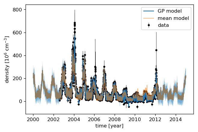
We can now calculate the “normal” (non-GP) model as well as the Gaussian Process prediction. Comparing the uncertainties to the data shows that the data variance amounts to roughly 10% of the data value. We therefore add 10% to the Gaussian Process predictive variance since we are predicting noisy targets.
[25]:
# Mean model prediction
mean_pred = model.get_value(times)

# GP predictive mean and variance
mu, var = gpmodel.predict(data, times, return_var=True)
# add 10% for noisy targets
std = np.sqrt(var + (0.1 * mu)**2)

plt.errorbar(time, data, yerr=2. * errs, fmt='.k', elinewidth=0.5, zorder=1, label="data")
plt.plot(times, mu, label="GP model")
plt.fill_between(times, mu - 2 * std, mu + 2 * std, alpha=0.6)
plt.plot(times, mean_pred, alpha=0.5, label="mean model")
plt.ylabel("density [10$^{{{0:.0f}}}$ ${1}$]"
           .format(-np.log10(data_scale), data_ts.NO_DENS.attrs["units"]))
plt.xlabel("time [year]")
plt.legend();
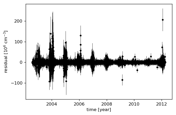
Let’s look at the residuals to see how well the model fits the data. We therefore “predict” the data at the measurement times.
[26]:
mu, var = gpmodel.predict(data, time, return_var=True)
# again, 10% for noisy targets
std = np.sqrt(var + (0.1 * mu)**2)

plt.errorbar(time, data - mu, yerr=2 * std, fmt='.k', elinewidth=0.5)
plt.ylabel("residual [10$^{{{0:.0f}}}$ ${1}$]"
           .format(-np.log10(data_scale), data_ts.NO_DENS.attrs["units"]))
plt.xlabel("time [year]");
MCMC sampling
The Markov-Chain Monte-Carlo sampling is done with emcee, and we set up the sampler to something that does not take too long on a single machine. You can change the number of walkers or increase the number of threads to speed up the sampling.
[27]:
import emcee

initial = gpmodel.get_parameter_vector()
ndim, nwalkers = len(initial), 48
p0 = initial + 1e-4 * np.random.randn(nwalkers, ndim)
sampler = emcee.EnsembleSampler(nwalkers, ndim, lpost, args=(data, gpmodel), threads=2)
[28]:
print("Running burn-in...")
p0, _, _ = sampler.run_mcmc(p0, 200)

sampler.reset()

print("Running production...")
sampler.run_mcmc(p0, 800);
Running burn-in...
Running production...
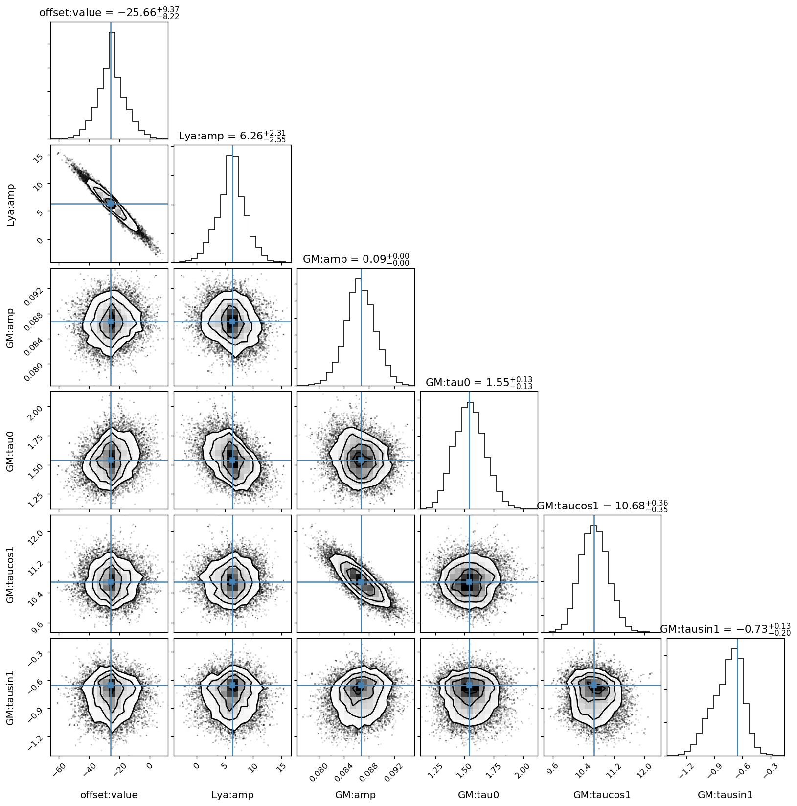
Sampled results
We use the corner module to plot the sampled parameter distributions.
[29]:
import corner

names = gpmodel.get_parameter_names()
cols = model.get_parameter_names()
# the indices of the mean model parameters
inds = np.array([names.index("mean:" + k) for k in cols])
This figure shows the sampled distributions of the mean model parameters only, excluding the Gaussian Process kernel’s parameters. The “true” values are taken from the scipy.optimize.minimize fit above.
[30]:
# only mean model parameters
corner.corner(sampler.flatchain[:, inds],
              show_titles=True,
              title_kwargs={"fontsize": 13},
              truths=res_opt.x[inds],
              label_kwargs={"fontsize": 12},
              labels=cols);
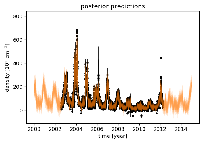
To have an idea about the variance of the predictions, we select a few samples from the paramter distributions which were just sampled by emcee. We then draw a random sample from the corresponding multivariate normal distribution with the predictive mean and covariance (plus the data variance) as parameters.
[31]:
# Plot the data.
plt.errorbar(time, data, yerr=2 * errs, fmt=".k", elinewidth=0.5, zorder=1, label="data")

# Plot 12 posterior samples.
samples = sampler.flatchain
for s in samples[np.random.randint(len(samples), size=12)]:
    gpmodel.set_parameter_vector(s)
    mu, cov = gpmodel.predict(data, times[::10])
    cov[np.diag_indices_from(cov)] += (0.1 * mu)**2
    sampl = np.random.multivariate_normal(mu, cov)
    plt.plot(times[::10], sampl, color="C1", alpha=0.1)

plt.ylabel("density [10$^{{{0:.0f}}}$ ${1}$]"
           .format(-np.log10(data_scale), data_ts.NO_DENS.attrs["units"]))
plt.xlabel("time [year]")
plt.title("posterior predictions");